Differential geometry is the language of cartography and also of general relativity, in addition to being a rich and beautiful mathematical theory in its own right. In a nutshell, this theory expands the standard theory of multi-variable and vector calculus to a space which is not necessarily “flat”. In this article we will construct the basic building blocks of this theory, based on the special case of the surface of a sphere.
The surface of a unit sphere
The unit sphere is the collection of all points in the 3-dimensional Euclidean space that are a unit distance from the origin:
$$
\mathcal{S}^2 = \{(x,y,z) \;\; | \;\; x^2 + y^2 + z^2 = 1\}
$$
Which we can visualize using the wonderful GeoGebra tool:

Other than being relatively simple while still having all the complexity required to develop the tools of differential geometry, the surface of the sphere has the added bonus of describing the world we live in. We’re all, to a good approximation, live on the surface of the sphere, so concepts like ‘poles’ and ‘geodesics’ bear intuitive understanding for us.
Our focus in this article will be on the northern hemisphere only, an object which will we refer to as a manifold. Our goal will be to calculate the length of a path on this manifold. To achieve this we will need to develop some of the basic mathematical tools which are at the foundations of differential geometry. Let’s get to it.
Coordinate maps
First we need a convenient way to represent points on our manifold, i.e. we need a coordinate system that will assign a unique label to each point on the northern hemisphere. Since the surface of the sphere is 2-dimensional, we will need two independent coordinates to achieve this. We will also want our coordinate system to be continuous: if two points are near each other on the sphere their coordinates should also be close to one another. Such a mapping is referred to as a coordinate chart, denoted as $\psi$, and in the general case it assigns points in a sub-region of the $m$-dimensional Euclidean space to an $m$-dimensional manifold. We also require that the mapping will be a bijection: it can represent any point on the manifold and any such point is described uniquely. This ensures that there is an inverse mapping, $\psi^{-1}$, which maps points from the manifold to the $\mathbb{R}^m$ coordinates. For our 2-dimensional manifold, we denote by $(x^1,x^2)$ any general coordinates of $\mathbb{R}^2$. The mapping function is $\psi: \mathbb{R}^2 \rightarrow \mathbb{R}^3$ and it consists of three separate functions $\mathbb{R}^2 \rightarrow \mathbb{R}$, one for each coordinate in $\mathbb{R}^3$:
$$
\psi(x^1,x^2) = (\psi^x(x^1,x^2), \psi^y(x^1,x^2), \psi^z(x^1,x^2))
$$
Let’s explore several such mappings. The first one will be very simple and straightforward – since we are interested only in the northern hemisphere of the unit sphere, we can simply use the Cartesian coordinates of the $x$-$y$ plane, which we will denote as $(X,Y)$, giving us a mapping from the surface of the sphere to the unit disc. The coordinate mapping in this case is given by:
$$
\psi(X,Y) = (X,Y,\sqrt{1-X^2-Y^2})
$$
We can also describe the same projection using polar coordinates $(r,\theta)$ which are given by:
$$
\begin{align}
r &= \sqrt{x^2 + y^2} \\
\theta &= \tan^{-1}(y/x)
\end{align}
$$
And the coordinate map in this case is given by:
$$
\psi(r,\theta) = (r\cos(\theta),r\sin(\theta),\sqrt{1-r^2})
$$
A third possible mapping is to use spherical coordinates $(\phi, \theta)$ which are defined as:
- $\phi \in [0,\pi/2]$ is the polar angle: the angle between a line connecting the point to the origin and the z-axis.
- $\theta \in [0,2\pi)$ is the azimuth angle: the angle between the x-axis and the line connecting the origin and the projection of the point to the $x$-$y$ plane. This is the same $\theta$ used in the polar coordinates (hence the identical notation)
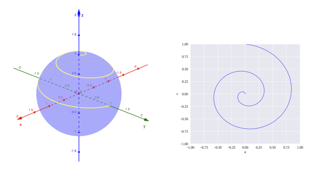
The fourth and final way is to use stereographic projection from the south pole. In this method we map a point $P$ on the sphere to a point $(u,v)$ on the $x$-$y$ plane by stretching a line from the south pole (the point $(0,0,-1)$) to the point $P$. The intersection of this line with the $x$-$y$ plane marks the point $(u,v)$ which is assigned to $P$.

The following table summarizes all the four mappings we defined:
| Mapping | Notation | $\psi$ | $\psi^{-1}$ |
|---|---|---|---|
| Cartesian | $(X,Y)$ | $(X,Y,\sqrt{1-X^2-Y^2})$ | $(x,y)$ |
| Polar | $(r,\theta)$ | $(r\cos(\theta),r\sin(\theta),\sqrt{1-r^2})$ | $(\sqrt{x^2+y^2},\tan^{-1}(y/x))$ |
| Spherical | $(\phi,\theta)$ | $(\sin(\phi)\cos(\theta),\sin(\phi)\sin(\theta),\cos(\phi))$ | $(\cos^{-1}(z),\tan^{-1}(y/x))$ |
| Stereographic | $(u,v)$ | $(2u, 2v, 1-u^2-v^2)/(1+u^2+v^2)$ | $(x/(1+z),y/(1+z))$ |
To get a feel of how the four mappings differ from one another, we can draw the same patch of area on the sphere as it is projected into each one of our coordinate maps:

We will move on to calculating path lengths using our coordinate maps.
Path length in Euclidean space
Before we analyze paths on the surface of the sphere, let’s first discuss paths in the regular Euclidean space $\mathbb{R}^2$ and the calculation of their length. A path is a smoothly connected set of points in space, with two end points. This is probably easiest described using a parametrization:
$$
R = \{ (x^1(t),x^2(t)) \;\; | \;\; t \in [t_0,t_1] \}
$$
Where $x^1(t)$ and $x^2(t)$ are smooth continuous functions.
We will start by simply working with the Cartesian coordinates $(x,y)$ directly. The basic formula from which everything else will be derived is the Euclidean distance formula, which is based on Pythagoras theorem. For two points $P_1=(x_1,y_1)$ and $P_2=(x_2,y_2)$, the Euclidean distance between them is:
$$
D = \sqrt{(x_2-x_1)^2+(y_2-y_1)^2} \tag{1}
$$
This calculation is already a specific case of path length – it is the length of the path of the straight line connecting the points $P_1$ and $P_2$, which we can describe parametrically as:
$$
R(t) = P_1 + t(P_2-P_1) \,\,\,\, t\in[0,1] \tag{2}
$$
For a general path, to calculate its length we can break it into small segments and add up their individual lengths. A small line segment, which we denote as $dR$, is the amount of “path” we need to add to get from $R(t)$ to $R(t+dt)$:
$$
R(t+dt) = R(t) + dR
$$
So to get the total path length we need to sum up all the lengths of the small $dR$ path segments. Since the path is smooth, we can assume that for $dt$ small enough each such segment is a straight line:
$$
R(t+dt) = R(t) + R'(t)dt
$$
The length of the path, which we denote as $L$, is therefore given by:
$$
L = \int||dR|| = \int_{t_0}^{t_1} ||R'(t)||dt = \int_{t_0}^{t_1} \sqrt{x'(t)^2 + y'(t)^2}dt \tag{3}
$$
It can be easily checked that for the case of a straight line (2), this expression gives the same result as (1).

What happens if we use a different coordinate system? Well, the path of course is the same path regardless of which coordinate system we choose to describe it with, so the length should come out the same, but what exactly do we need to integrate to get the correct answer? Let’s analyze this by using the example of polar coordinates, in which we can parametrize our path as follows:
$$
R = \{ (r(t),\theta(t)) \;\; | \;\; t \in [t_0,t_1] \}
$$
Since both Cartesian and polar coordinates are valid coordinate systems which uniquely describe each point in $\mathbb{R}^2$, we can switch between them as we want. But since we’ve already solved things out in the Cartesian case, we can use it to figure out the proper method in the polar coordinates case. If we could express the derivatives $x’$ and $y’$ in terms of $r’$ and $\theta’$, then we can substitute them into (3) and get the expression for the path length in polar coordinates. To do this, let’s first recall the formulas for converting from polar coordinates to Cartesian coordinates:
| Coordinate | Calculation | $\partial / \partial r$ | $\partial / \partial \theta$ |
|---|---|---|---|
| $x$ | $r\cos(\theta)$ | $\cos(\theta)$ | $-r\sin(\theta)$ |
| $y$ | $r\sin(\theta)$ | $\sin(\theta)$ | $r\cos(\theta)$ |
If we differentiate the $(x,y)$ coordinates with respect to $t$ by going through their expressions in terms of $(r,\theta)$ we get:
$$
\begin{align}
x’ = &\frac{dx}{dt} = \frac{\partial x}{\partial r}\frac{dr}{dt} + \frac{\partial x}{\partial \theta}\frac{d\theta}{dt} = \cos(\theta)r’ – r\sin(\theta)\theta’ \\
y’ = &\frac{dy}{dt} = \frac{\partial y}{\partial r}\frac{dr}{dt} + \frac{\partial y}{\partial \theta}\frac{d\theta}{dt} = \sin(\theta)r’ + r\cos(\theta)\theta’
\end{align}
$$
And now we can substitute this into (3) and get:
$$
L = \int_{t_0}^{t_1} \sqrt{r'(t)^2 + r(t)^2\theta'(t)^2}dt \tag{4}
$$
Which looks very similar to (3), except now the second coordinate picked up the scaling factor $r(t)$.
It’s natural at this point to try and generalize this process for any transition between different coordinate systems, but for now we’re going to leave this discussion at this point and move on to calculate the length of a path on the surface of the sphere, which as we will see is in a sense a different kind of generalization.
Path length on a sphere
We will denote by $R_3(t)$ a path $(x(t),y(t),z(t))$ which lies entirely on our manifold. Using a given coordinate chart we can describe $R_3(t)$ from a corresponding path $R(t)$ in $\mathbb{R}^2$, which we denote as $(x^1(t),x^2(t))$:
This “projected path” looks exactly like our general path in $\mathbb{R}^2$ from the previous discussion, and we would like to find an expression that allows us to use a similar integral on this path that will get us the length of $R_3$. We can again do this by breaking $R(t)$ into small segments and summing their lengths, but for this we need to figure out what is the ‘local length’ of $R_3(t)$ at any point $t$ along the path, which we denote as $||dR_3||$. As before, we can find $dR_3$ in terms of our $\mathbb{R}^2$ coordinates using standard derivation rules as follows:
$$
\begin{align}
dR_3 &= R_3(t+dt) – R_3(t) \\
&= R’_3 (t)dt \\
&= (x'(t), y'(t), z'(t)) dt \\
&= (x'(x^1(t),x^2(t)), y'(x^1(t),x^2(t)), z'(x^1(t),x^2(t))) dt \\
&= \left(\frac{\partial \psi^x}{\partial x^1}\frac{dx^1}{dt}+\frac{\partial \psi^x}{\partial x^2}\frac{dx^2}{dt}, \frac{\partial \psi^y}{\partial x^1}\frac{dx^1}{dt}+\frac{\partial \psi^y}{\partial x^2}\frac{dx^2}{dt}, \frac{\partial \psi^z}{\partial x^1}\frac{dx^1}{dt}+\frac{\partial \psi^z}{\partial x^2}\frac{dx^2}{dt}\right)dt
\end{align}
$$
The calculation certainly gets quite involved, but it’s worth emphasizing that although somewhat abbreviated, every term in the expression above is ultimately a function of $t$. For example, we can explicitly write:
$$
\frac{\partial \psi^x}{\partial x^1} = \frac{\partial \psi^x}{\partial x^1}(x^1(t),x^2(t))
$$
Since our goal is to find the correct length integral in $\mathbb{R}^2$, it would help to isolate the derivatives $(x^1)’$ and $(x^2)’$, which we can do by continuing the development as follows:
$$
\begin{align}dR_3 &= \left[
\left(\frac{\partial \psi^x}{\partial x^1},\frac{\partial \psi^y}{\partial x^1},\frac{\partial \psi^z}{\partial x^1}\right)\frac{dx^1}{dt} +
\left(\frac{\partial \psi^x}{\partial x^2},\frac{\partial \psi^y}{\partial x^2},\frac{\partial \psi^z}{\partial x^2}\right)\frac{dx^2}{dt}
\right] dt
\end{align}
$$
This path segment is a vector in the 3-dimensional Euclidean space, so we can use the Euclidean distance formula to calculate its length, which comes out to:
$$
\begin{align} ||dR_3||^2 = &\left[ \left(\frac{\partial \psi^x}{\partial x^1}\right)^2 + \left(\frac{\partial \psi^y}{\partial x^1}\right)^2 + \left(\frac{\partial \psi^z}{\partial x^1}\right)^2\right] \left(\frac{dx^1}{dt}\right)^2 dt^2\\
&\left[ \left(\frac{\partial \psi^x}{\partial x^2}\right)^2 + \left(\frac{\partial \psi^y}{\partial x^2}\right)^2 + \left(\frac{\partial \psi^z}{\partial x^2}\right)^2\right] \left(\frac{dx^2}{dt}\right)^2 dt^2\\
&\left[ \frac{\partial \psi^x}{\partial x^1}\frac{\partial \psi^x}{\partial x^2} + \frac{\partial \psi^y}{\partial x^1}\frac{\partial \psi^y}{\partial x^2} + \frac{\partial \psi^z}{\partial x^1}\frac{\partial \psi^z}{\partial x^2}\right]2\frac{dx^1}{dt}\frac{dx^2}{dt} dt^2
\end{align}
$$
To finish things up, let’s use some notation to make this expression more succinct. We will denote by $g_{11}$ the coefficient attached to the $x^1$ coordinate, by $g_{22}$ the coefficient attached to the $x^2$ coordinate and by $g_{12}$ and $g_{21}$ each half the coefficient attached to the cross term. With this notation we can write $||dR_3||^2$ as:
$$
||dR_3||^2 = \left[g_{11}\left(\frac{dx^1}{dt}\right)^2 + g_{22}\left(\frac{dx^2}{dt}\right)^2 + g_{12}\left(\frac{dx^1}{dt}\frac{dx^2}{dt}\right) + g_{21}\left(\frac{dx^2}{dt}\frac{dx^1}{dt}\right)\right]dt^2 \tag{5}
$$
And we can now finally write down the length integral using our chosen coordinate system as:
$$
L = \int_{t_0}^{t_1} \sqrt{g_{11}\left(\frac{dx^1}{dt}\right)^2 + g_{22}\left(\frac{dx^2}{dt}\right)^2 + g_{12}\left(\frac{dx^1}{dt}\frac{dx^2}{dt}\right) + g_{21}\left(\frac{dx^2}{dt}\frac{dx^1}{dt}\right)}dt \tag{6}
$$
If we compare (6) to (3) and (4) we can again see that there is some resemblance between them. In this case however we get scaling coefficients for both coordinates, and additional cross terms which now appeared. Let’s now try to make sense of it all.
Path length from a different perspective
Looking again at equation (6), we can see that it generalizes both equations (3) and (4). If we arrange the $g_{ij}$ coefficients in a 2×2 matrix, we get that for equation (3) this matrix is the identity matrix, and for equation (4) this matrix is given by:
$$
g = \left[ \begin{matrix} 1 & 0 \\ 0 & r\end{matrix} \right]
$$
But what is the role this matrix takes? In all the cases we’ve explored, to find the length of a path segment at a point $t$ along our $\mathbb{R}^2$ path we took the following steps:
- We calculated the coordinate translation vector in $\mathbb{R}^2$ which is given by: $dx = ((x^1)’dt, (x^2)’dt)$
- We used equation (5) to transform $dx$ into the actual length we are interested in
In the case of equation (3), the calculation in step 2 is simply the norm of the coordinate translation vector $dx$, which is the inner product of the vector with itself. So the matrix $g$ can be thought of as generalizing the notion of inner product of vectors. If the standard inner product of two vectors $u = (u_1,u_2)$, $v=(v_1,v_2)$ is given by:
$$
\langle u,v \rangle = u_1v_1 + u_2v_2 = u^Tv
$$
In our new framework the inner product takes the form:
$$
\langle u,v \rangle = u^Tgv
$$
Another way to think about this is that our chosen coordinate system always looks like $\mathbb{R}^2$, but it doesn’t necessarily describes $\mathbb{R}^2$. Instead it describes a “real” 2-dimensional space, and the matrix $g$, which takes some value at any point on our map, tells us how lengths are measured in the real space at that point. In the case of coordinate change in $\mathbb{R}^2$ the “real” space is $\mathbb{R}^2$ itself, but the coordinates we use, for example polar coordinates, don’t describe $\mathbb{R}^2$ directly but rather require some transformation $g$ to translate lengths on the map to real $\mathbb{R}^2$ lengths.
The matrix $g$ is one of the most fundamental entities in differential geometry and is known as the metric tensor. We of course need to first define what is a tensor in order to rationalize this name, which will be the topic of a future article in this series. In the next article, we will explore angles and areas on manifolds, and we will again see how the metric tensor takes a role in these also.
Epilogue – some examples of metric tensors
As we’ve invested so much work in developing general formulas for the metric tensor of the northern hemisphere manifold, it could be nice to see what actual expressions we get for this metric tensor under different coordinate charts. Recall that the metric tensor coefficients are given by:
$$
\begin{align}
g_{11} &= \left(\frac{\partial \psi^x}{\partial x^1}\right)^2 + \left(\frac{\partial \psi^y}{\partial x^1}\right)^2 + \left(\frac{\partial \psi^z}{\partial x^1}\right)^2 \\
g_{22} &= \left(\frac{\partial \psi^x}{\partial x^2}\right)^2 + \left(\frac{\partial \psi^y}{\partial x^2}\right)^2 + \left(\frac{\partial \psi^z}{\partial x^2}\right)^2 \\
g_{12} &= \frac{\partial \psi^x}{\partial x^1}\frac{\partial \psi^x}{\partial x^2} + \frac{\partial \psi^y}{\partial x^1}\frac{\partial \psi^y}{\partial x^2} + \frac{\partial \psi^z}{\partial x^1}\frac{\partial \psi^z}{\partial x^2}
\end{align}
$$
And we also have $g_{21} = g_{12}$.
Using the Cartesian map $(X,Y)$ we get that the metric tensor becomes:
$$
g(X,Y) = \frac{1}{1-X^2-Y^2} \left[ \begin{matrix} 1-Y^2 & XY \\ XY & 1-X^2\end{matrix} \right]
$$
Using the Spherical map $(\phi,\theta)$ we get that the metric tensor becomes:
$$
g(\phi,\theta) = \left[ \begin{matrix} \cos(2\phi) & 0 \\ 0 & \sin^2(\phi)\end{matrix} \right]
$$