Alice is texting Bob, telling him she has to stay late at work and asking him if he could pick up the kids from soccer practice. Bob replies that sure, he can move some things around and make it. Love you. Love you too.
In this interaction, what is it exactly that passed from Alice to Bob and vice versa, causing them to change their actions? Physically, it was electric pulses moving by air and cables, processed by microchips and converted to symbols displayed on screens. But this is not the essence of it. Other mediums could have been used instead: conversation in the form of vibrating air pressure, written words on a paper, smoke signals, etc. The essence here is not the physical process that was used, but rather the information – it was information that passed between them, that is really important. But what is information? Is it possible to quantify it? Well, turns out it is indeed possible, as was shown by Claude Shannon in 1948.
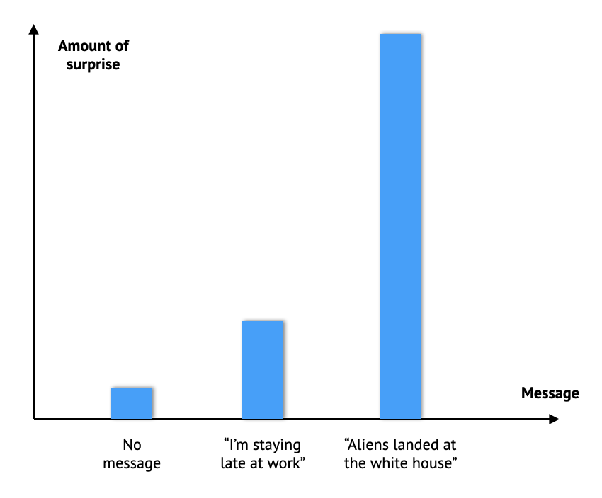
To do this, let’s think about what it means for Bob to receive a message from Alice. We can imagine all the possible messages Alice could send Bob, and for completeness let’s include the “no message” as a kind of message as well. For each such message we can start by asking ourselves the somewhat odd question: “how much this message would surprise Bob”? The “no message” message for example would probably not surprise Bob very much, as typically he would not expect to receive a message from Alice. On the other hand, if he were to receive the message “An alien spaceship has just landed in front of the white house”, he would probably be very surprised (assuming he did not already hear about this in the news). The message “I have to stay late at work” lies somewhere in between. So we can certainly rank the messages according to how much they would surprise Bob:
The mental leap we will do now is to link the notion of “surprise” to the notion of “information”, and we will do this by stating that the amount of information a given message has conveyed is proportional to the surprise the message has caused the recipient.
Can we quantify this? Well, luckily, probability theory provides us with the mathematical tools we need to do so.
Quantifying information
As a start, we can formalize our hand wavy notion of surprise by asking Bob to assign a probability to every possible message he can receive from Alice:
$$p_i=\Pr\left( \text{message i} \right)$$
These probabilities reflect the likelihood Bob assigns to receiving any specific message – the lower the probability of a message, the more surprised Bob would be to receive that message. Here, we think of Alice as an information source, which can be modeled as a random variable $X$ taking values (messages) $x_i$ with probabilities $p_i$. What we would like to have is some kind of notion of ‘information’ $I_i$, assigned to the message $x_i$, which is inversely proportional to $p_i$. Also, we would like for the values taken by this measure to span the range of 0 (no information) to infinity (infinite information). Since each $p_i$ is between 0 and 1, a simple such measure is given by:
$I_i = -\log_2 \left( p_i \right)$
It is reasonable to consider other functions that satisfy the conditions above, however the logarithm function has some convenient properties which makes it attractive in this case, as we will see later. The reason that the logarithm is taken in base 2 is somewhat arbitrary, and other bases can be used as well. Regardless, as long as base 2 is used we assign the unit of bits to the information measure $I_i$. From now on we will just use the notation $\log$ instead of \$log_2$.
Now that we defined the so called ‘self information’ of the message $x_i$, we can calculate the mean value of the information of all messages, which is denoted as $H$:
$H = E\left[ I \right] = -\sum_ip_i\log \left( p_i \right)$
This measure is one of the key concepts of information theory, and is referred to as the entropy of the random variable $X$. Freely speaking, the entropy measures how disordered the variable $X$ is. If for example $X$ is deterministic, meaning it generates a single value with probability 1, then the entropy of $X$ will be 0. For any other case the entropy will be greater than 0. One of the main reasons for why the notion of entropy is so important in information theory is that this measure answers a very practical question about the random variable $X$, which is: ‘how many bits are required to encode the messages produced by $X$?’. The rest of this article is dedicated to answering this very question.
As a side note, it’s worth noting that the entropy does not depend at all on the values $X$ takes, but only on their probabilities. Particularly, $X$ does not even have to take on numerical values. This is a key feature of information theory, which unlike basic probability theory or statistics where we often analyze quantities like the mean and variance of random variables, which depend on both the values taken by a random variable and their probabilities, in information theory we only care about the probabilities, making this theory somewhat more abstract.
Typicality
To make our analysis easier, we will replace Alice with a simpler information source – a biased coin, which we will denote as $X$. Whenever our coin is being tossed it has a probability of $0.9$ to land on Heads ($p_H = 0.9$) and a probability $0.1$ to land on Tails ($p_T = 0.1$). The entropy of this biased coin toss random variable is:
$H(X) = -0.1\log(0.1) – 0.9\log(0.9) \approx 0.469 \;\; [\text{bits}]$
Suppose Alice has tossed the coin $n$ times, each time recording the result. Now she wants to send the sequence she recorded to Bob (we can think of each result as a message Alice sends Bob, thus simplifying the original setup into one where there are only two types of messages, with probabilities $0.1$ and $0.9$). To do this, she can can assign the digit 0 to the result ‘Heads’ and the digit 1 to the result ‘Tails’, and then write the recorded sequence on a piece of paper as a sequence of 1’s and 0’s and send the piece of paper to Bob. To decipher the sequence, Bob will of course need to know that 0 means ‘Heads’ and 1 means ‘Tails’, and using this knowledge and the piece of paper sent from Alice he can recover the sequence of coin toss results. This procedure of converting the information into a sequence of binary digits, or bits for short, is referred to as coding. A given sequence that Alice sends is referred to as a codeword, and the entire set of possible codewords is simply referred to as a code. The process of converting the information into a codeword is referred to as encoding, and the sequence of converting a codeword back into the original information is referred to as decoding. It is always assumed that both parties are aware of the code that’s being used, and can therefore exchange information between them using encoding and decoding.
How many bits will Alice have to write down on the paper? Well, the answer seems rather obvious – there are $n$ coin toss results, so she would need $n$ bits. But as it turns out, this is rather wasteful. With some proper planning, Alice can reduce the number of bits to less than 50% of $n$ and still convey all the information of the sequence, given that $n$ is long enough. To understand why, let’s analyze the sequences our biased coin can produce.
Let’s denote a sequence of $n$ coin toss results as $\underline{x}$:
$\underline{x} = \left( x_1, x_2, …,x_n \right)$
There are $2^n$ possible such sequences. Which one is the most likely one? Well, since at each toss it’s more likely the coin will land on Heads, the most likely sequence is the sequence of all Heads, which has probability:
$\Pr \left( \text{all Heads}\right) = 0.9^n$
But is this the sequence we expect to see? Lets think about it for a moment. We know that Tails has probability of $0.1$ to show up, so within $n$ coin tosses we would expect about 10% of them to come up as Tails, and about 90% to come up as Heads. The probability of seeing a specific such ‘typical sequence’ is given by:
$\Pr \left( \text{typical sequence}\right) = 0.9^{0.9n}\cdot 0.1^{0.1n}$
(This expression technically assumes that $0.1n$ is an integer, but we can ignore this for now by rounding anything as necessary, and treating the resulting calculation as an approximation). This probability is of course lower than the probability of the sequence of all Heads, so how can we justify the fact that we would expect to see such a sequence? The straight forward answer is that there are many such sequences, in fact, there are $\binom{n}{0.1n}$ such sequences, while there is only one sequence of all Heads. But to help us make this more formal, we will switch from analyzing the probability of a given sequence to analyzing the entropy of a given sequence, which is given by:
$\hat{H}(\underline{x}) = \frac{-\log(\Pr(\underline{x}))}{n} = -\frac{1}{n}\sum_{j=1}^{n}\log (\Pr(x_j))$
This quantity is the empirical counterpart of the entropy of the random variable $X$, much like how the average of a sequence of random outcomes of a random variable is an empirical estimation for the mean value of that random variable. The table below compares the probability and entropy of the most likely and typical sequences:
| Sequence | Type | Probability | Entropy | Entropy [bits] |
|---|---|---|---|---|
| All Heads | Most likely | $0.9^n$ | $-\log(0.9)$ | 0.152 |
| 10% Tails, 90% Heads | Typical | $0.9^{0.9n}\cdot 0.1^{0.1n}$ | $-0.1\log(0.1)-0.9\log(0.9)$ | 0.469 |
We notice something interesting – even though the most likely sequence has the maximal probability, the typical sequence has higher entropy, which is also equal to the entropy of $X$. Up until now we’ve only analyzed two types of sequences – the sequence of repeated Heads and the sequences containing exactly 10% Tails. There are of course many other possible sequences, and motivated by our observations we would now like to divide them into two groups: the ‘typical set’, which contains all the sequences which are close to the typical sequence, and the rest of the sequences. For a length $n$ sequence and a positive $\epsilon$ the typical set is formally defined as:
$A_n^{\epsilon} = \{ \underline{x} : | \hat{H}(\underline{x}) – H(X) | < \epsilon \}$
Which simply means that we include in this set all sequences whose empirical entropy is no more than $\epsilon$ away from the entropy of $X$. We are free to choose $\epsilon$ to be as small as we want, but nevertheless we expect that for large enough $n$ the sequence we will observe in practice will be one of the sequences in this set. This is what we will now show.
Asymptotic equipartition
There are two things we want to show about our typical set:
- The probability that an observed sequence will be from the typical set is close to 1
- All sequences in the typical set roughly have the same probability
The second statement is one that we’ve not discussed so far, but as it turns out, it is both true and useful. Put together, these statements are known as the Asymptotic Equipartition property, or AEP for short, and is arguably the most fundamental concept in information theory.
The mathematical tool we will use is the weak version of the Law of Large Numbers (LLN). This law, which we will not prove, states that if we have:
- A random variable $Z$ with expected value $E[Z]$
- A length $n$ sequence $\underline{z}$ of realizations of $Z$
Then we can choose any $\epsilon > 0$ as small as we want and any $\delta > 0$ as small as we want, and we are guaranteed that there exists a large enough $n$ such that with probability at least $1-\delta$ the gap between the average of $\underline{z}$ and $E[Z]$ is less than $\epsilon$. This can be written more succinctly as:
$\lim_{n \rightarrow \infty} \Pr\left( \left| \bar{z} – E[Z] \right| < \epsilon \right) = 1$
Where $\bar{z}$ is the average of $\underline{z}$. We can apply this law to our example – if we replace Heads with 0 and Tails with 1, then the expected value of a coin toss is:
$E[X] = 0.9 \cdot 0 + 0.1 \cdot 1 = 0.1$
The LLN tells us that if we average the values in a sequence of coin tosses, then with high probability this average will be as close to 0.1 as we want, assuming $n$ is large enough. The clever trick we will use to prove the AEP property is to convert our random variable $X$ into another random variable $Y$ which is given by:
$Y = -\log(\Pr(X))$
Remember that $\Pr()$ is just a function that takes values of $X$ and assigns them numbers between $0$ and $1$, so $Y$ is a well defined random variable. The expected value of $Y$ is equal to the entropy of $X$ since:
$E[Y] = -\sum_i p_i\log(p_i) = H(X)$
Going back to our sequence $\underline{x}$, we recall that its entropy is given by:
$\hat{H}(\underline{x}) = \frac{-\log(\Pr(\underline{x}))}{n} = \frac{1}{n}\sum_{n=1}^{n}[-\log (\Pr(x_n))]$
But this quantity is nothing more than the average of a sequence of realizations of $Y$, so by applying the LLN on $Y$ we get that:
$\lim_{n \rightarrow \infty} \Pr\left( \left| \hat{H}(\underline{x}) – H(X) \right| < \epsilon \right) = 1$
Which according to the way we’ve constructed the typical set is equivalent to:
$\lim_{n \rightarrow \infty} \Pr\left( \underline{x} \in A_n^{\epsilon} \right) = 1$
Which proves the first statement.
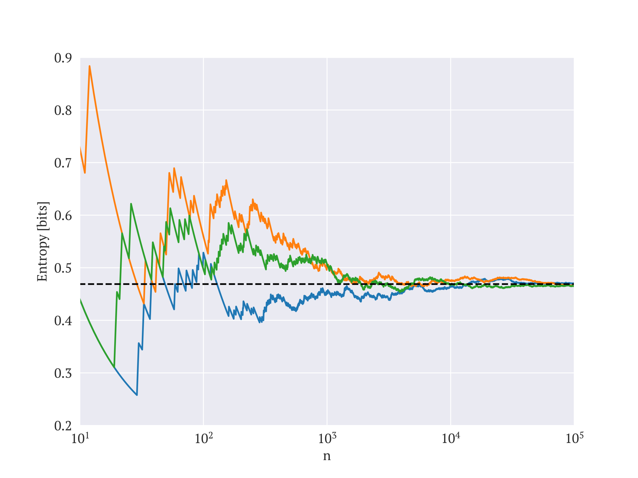
To illustrate the entropy convergence, the figure below shows the entropy of three randomly generated sequences of 100,000 toss results of our biased coin. The value of the graph at each point is the entropy calculated using the first $n$ entries in the sequence. We can see that the convergence is not very fast, as a few thousands of realizations are required to get a descent approximation to $H(X)$. Regardless, it also shows that indeed the empirical entropy does eventually converges to the theoretical one.
Now let’s go back to our typical set and write it as follows:
$A_n^{\epsilon} = \{ \underline{x} : -\epsilon < \frac{-\log(\Pr(\underline{x}))}{n} – H(X) < \epsilon \}$
By rearranging the expression a bit we can write it as:
$A_n^{\epsilon} = \{ \underline{x} : 2^{-n(H(X)+\epsilon)} < \Pr(\underline{x}) < 2^{-n(H(X)-\epsilon)} \}$
Which tells us that all sequences in the typical set roughly have the same probability which is:
$\Pr(\underline{x}) \approx 2^{-nH(X)}$
As asserted by the second statement.
Compressing data
Let’s continue our hand wavy calculations a bit further. For an arbitrary large value of $n$, we have a typical set of sequences, each one has probability of about $2^{-nH(x)}$ to come up, and all of them together have a joint probability of about 1. By dividing both numbers, we can deduce how many sequences there are in the typical set:
$|A_n^{\epsilon}| \approx \frac{\Pr(A_n^{\epsilon})}{\Pr(\underline{x} | \underline{x} \in A_n^{\epsilon})} \approx \frac{1}{2^{-nH(x)}} = 2^{nH(X)}$
In our biased coin example there are $2^n$ possible sequences, so the relative size of the typical set compared to the entire sequence space is:
$\frac{2^{nH(x)}}{2^n} = 2^{n(H(X)-1)}$
Since $H(X) < 1$, as $n$ gets larger the relative size of the typical set compared to the entire sequence space becomes vanishingly small, although it still holds most of the probability. This feature of the typical set is what enables us to compress the sequence data: suppose we generated a sequence and we want to send or store it using as little number of bits as possible. Since it’s very likely the sequence we have comes from the typical set, instead of worrying about how to represent a general length $n$ sequence, we only need to worry about how to represent a length $n$ typical sequence. But since there are much fewer typical sequences than general sequences, we need much fewer bits to distinguish between them. In general, the number of bits we need to represent an element from a set of $K$ elements is $\log(K)$, so the number of bits we need to represent a sequence from the typical set is:
$\log|A_n^{\epsilon}| \approx nH(X)$
In our biased coin example, where $H(X) \approx 0.47$, this translates to more than 50% reduction compared to the number of bits we would need if we were to just write down the result of each toss like we did earlier. If we compare the number of bits used in the compressed version to the number of bits in the un-compressed version, we get the compression rate $R$ which is:
$R = \frac{nH(X)}{n} = H(X)$
The source coding theorem, which is the main goal of this article, states that for a random variable $X$ with entropy $H(X)$, there exists a code family such that as $n$ goes to infinity, the average codeword length for encoding a length $n$ sequence of realizations of $X$ approaches $nH(X)$. The discussion up until now showed why this is true, but we didn’t really prove this formally as there was a lot of hand waving going on. Let’s now fix this by constructing an explicit code and showing it achieves the desired compression rate. The proof is taken from the book “Elements of Information Theory” by Thomas M. Cover and Joy A. Thomas.
As a first step, we can upper bound the number of elements in the typical set. The minimal probability of a sequence in the typical set is:
$p_{min} = 2^{-n(H(X)+\epsilon)}$
Conversely, the probability of the entire typical set is upper bounded by 1. By dividing the two we can get an upper bound for the total number of elements in the typical set:
$|A_n^{\epsilon}| \leq 2^{n(H(X)+\epsilon)}$
The number of bits required to represent an element in the typical set, which we’ll denote as $n_0$, is therefore bounded above by:
$n_0 \leq \lceil \log 2^{n(H(X)+\epsilon)} \rceil = \lceil n(H(X)+\epsilon) \rceil$
We will now construct a code that maps a given length $n$ sequence $\underline{x}$ into a codeword $c(\underline{x})$. To do this, first we will assign a unique length $n_0$ bit label to each sequence in the typical set. Next, we will assign a unique length $n$ bit label to each sequence which is not in the typical set. Lastly, we will use a single bit to identify whether the sequence $\underline{x}$ is typical or not. This bit will be the first bit of the codeword, followed by the label of the sequence. This encoding ensures that a recipient can always recover $\underline{x}$. Overall, we used $n_0+1$ bits to encode a typical sequence and $n+1$ bits to encode a non-typical sequence. We will denote by $L$ the length of a codeword, which is a random variable that is given by:
$L = \begin{cases} n_0+1 & \underline{x} \in A_n^{\epsilon} \\ n+1 & \underline{x} \notin A_n^{\epsilon} \end{cases}$
All that’s left to do is to calculate the expected value of $L$, which is the average codeword length we will send:
$\begin{align} E[L] &= (n_0+1) \Pr(\underline{x} \in A_n^{\epsilon}) + (n+1) \Pr( \underline{x} \notin A_n^{\epsilon} ) \\
& \leq \left( \lceil n(H(X)+\epsilon) \rceil + 1 \right) (1-\delta) + (n+1)\delta \\
& \leq nH(X) + n\epsilon + 2 + \delta(n – nH(X) – n\epsilon – 1) \end{align}$
The compression rate we achieve with this code is:
$\begin{align} R &= \frac{E[L]}{n} \\
&\leq \frac{nH(X) + n\epsilon + 2 + \delta(n- nH(X) – n\epsilon – 1)}{n} \\
&= H(X) + \epsilon + \frac{2}{n} + \delta(1 – H(X) – \epsilon – 1/n) \end{align}$
Since both $\delta$ and $\epsilon$ are arbitrary, we are free to choose $\delta = \epsilon$, which simplifies the above to:
$R \leq H(X) + \frac{2}{n} + \epsilon(2 – H(X) – \epsilon – 1/n)$
This shows that by choosing $\epsilon$ as small as we want and letting $n$ be large enough, we can get a code rate which is as close as we want to $H(X)$, thus proving the source coding theorem.
Can we do better?
We have showed that we can find a compression code that will achieve the entropy rate. Can we find a better code, one that will achieve an even lower compression rate? We already saw that the best strategy is to focus on the typical set, and ignore everything outside it as it has vanishingly small probability to show up as $n$ grows larger. So the question really is whether there is redundancy inside the typical set, is there a subset in it that still holds all the probability while having considerably smaller size? The answer to this question is no. We will not prove this very carefully, but to see why let’s suppose we have another set $B_n^{\epsilon}$ that holds most of the probability. Since both $A_n^{\epsilon}$ and $B_n^{\epsilon}$ hold most of the probability, their intersection also must hold most of the probability, which means most of the members of $A_n^{\epsilon}$ are also members of $B_n^{\epsilon}$. But since a member of $A_n^{\epsilon}$ has probability of about $2^{-nH(X)}$ and most of them are members of $B_n^{\epsilon}$, this implies that $A_n^{\epsilon}$ and $B_n^{\epsilon}$ have the same size. Again, this is not a formal proof, but these statements can be made more accurate, and thereby ultimately proving that we cannot go below the entropy rate when we try to compress long sequences of data.
Closing remarks
We’ve introduced in this article several concepts such as entropy, coding, typical set, asymptotic equipartition, compression rate and more. These are all fundamental concepts of information theory, and many more results in this field are constructed based on them. One particular corner stone of information theory that is worth mentioning is the channel coding theorem, which gives an upper bound on the information rate that can be transmitted over a noisy communication channel. This theorem was the subject of the original 1948 paper by Shannon, “a mathematical theory of communication”, in which he first introduced the framework which is now known as information theory. Hopefully this theorem will be the topic of a future article.
Regardless, the source coding theorem which we proved here is also considered a corner stone of information theory, and is the basis for many practical compression problems and compression codes which are widely used these days. It’s worth emphasizing that although our proof of the source coding theorem was based on an explicit code which is well defined, in practice this is not a code that can actually be used. The reason is that an arbitrary enumeration of all elements in an exponentially growing set is infeasible. Instead, more efficient encoding and decoding algorithms were developed over time to allow a practical compression scheme for long sequences of data, which benefit from the low entropy of an information source.
There are of course quite a few questions that we’ve not addressed, for instance: What happens if the random variable we want to compress is continuous and not discrete? What happens if the sequence we want to compress is also continuous? What happens if the sequence we want to compress is not i.i.d (different messages can have statistical correlation)? These are some of the questions that drove the development of information theory over the years. The basic ingredients to answering them are, however, the ones we covered here.